How Do You Do A Tick On Excel

Hey there, fellow spreadsheet wranglers! So, you’ve found yourself in a bit of a pickle, huh? You're staring at your Excel sheet, and suddenly, a wild tick appears. What in the digital world is going on? Don't panic! It's not a rogue insect that’s somehow infiltrated your data, thank goodness. It’s actually a pretty cool little symbol, and once you know how to tame it, you’ll wonder how you ever lived without it. Think of me as your friendly neighborhood Excel guide, armed with coffee and a whole lot of patience.

First things first, let’s ditch the spooky movie vibe. That “tick” you’re seeing? It’s probably not a tick at all, unless you’re working with some very unusual data. More likely, you’ve stumbled upon what Excel calls a checkmark or a tick mark. It’s that little V-shaped symbol that usually means "yes," "done," "correct," or "approved." You know, the one you’d doodle in the margins of your old school notebooks when you aced a pop quiz? Yep, that one. Except now, it’s digital and way more official.

So, how do we summon this magical symbol into our spreadsheets? It’s not as complicated as deciphering a cryptic crossword puzzle, I promise. There are a few ways to go about it, and honestly, it depends on what you’re trying to achieve. Are you trying to mark tasks as complete? Are you creating a survey and want a simple way to indicate a choice? Or are you just feeling fancy and want to add a little flair to your data? We’ve got you covered.

Let's start with the most common scenario: you want to manually insert a tick mark. This is like picking up a pen and drawing it yourself, but with a keyboard. The easiest way, and the one I usually reach for first when I’m in a hurry (which, let’s be honest, is always), is by using the Character Map. Ever heard of it? It’s a hidden gem within Windows that holds all the symbols you could ever dream of. Seriously, it’s like a secret society of dingbats and special characters.

To get to it, you just need to do a quick search for “Character Map” in your Windows search bar. Poof! There it is. Now, this is where things get a little bit like a treasure hunt. You’ll need to scroll through a gazillion characters until you find that perfect tick. It can feel a bit overwhelming at first, like staring into the abyss of an ancient library. But trust me, it's in there!

Once you spot your coveted tick, you just click on it, hit "Select," and then "Copy." Now, hop back over to your Excel sheet, click in the cell where you want your tick to live, and hit "Paste." Ta-da! Instant satisfaction. You’ve just manually inserted a tick mark. High five! It’s a bit of a manual process, sure, but it’s foolproof once you know the trick. Think of it as a little workout for your mouse skills.

But wait, there's more! What if you need to do this for a lot of cells? Copy-pasting a hundred ticks can feel like digital torture. That's where Excel's built-in features come to the rescue, like a knight in shining armor. One of my absolute favorites is using the Wingdings font. Have you ever played around with that font? It’s a wild ride! It turns all your letters and numbers into little symbols and pictures. It’s like the alphabet decided to go on vacation and sent back postcards of icons.

So, here’s the magic: if you change the font of a cell to Wingdings (or even Wingdings 2 or Wingdings 3, because variety is the spice of life, right?), a specific character will turn into a tick mark. The most common character that transforms into a tick is the letter 'ü'. So, if you type 'ü' into a cell and then change the font to Wingdings, bam! You’ve got a tick. It’s like a secret code, and you’re now in on it. Isn’t that neat?

You can even copy and paste that 'ü' into multiple cells and then select all of them and change the font to Wingdings. All at once! See? We're getting faster already. This is perfect for creating simple checklists or marking items. Imagine, an entire column of checked items with just a few clicks and a font change. Efficiency, my friends, efficiency!

Now, what if you want something a bit more… dynamic? What if you want the tick to appear automatically based on some other data in your sheet? This is where we get into the fancy stuff, the realm of Excel formulas. Don't let it scare you; it's more like baking a cake than performing brain surgery. We're just mixing a few ingredients (formulas) to get a delicious result (a tick!).

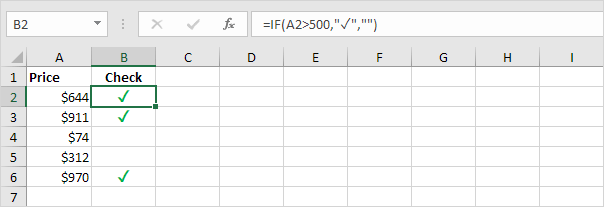
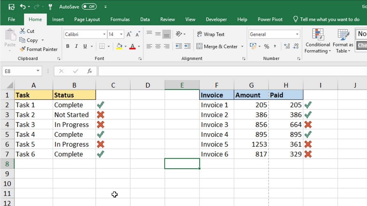
One of the most common ways to do this is using the IF function. It's a workhorse, this IF function. It basically says, "IF this condition is true, THEN do this, otherwise, ELSE do that." Simple, right? So, let's say you have a column where you type "Yes" or "No" for a task. You want a tick to appear next to "Yes" and maybe a cross next to "No," or perhaps just an empty cell. This is where IF shines.

You could write a formula like this: `=IF(A1="Yes", "ü", "")`. Let’s break that down, shall we? It means: IF the content of cell A1 is exactly "Yes", THEN put a 'ü' in this cell (which we'll then format as Wingdings), ELSE leave this cell blank (""). So, if you type "Yes" in A1, a tick appears. If you type "No" or anything else, the cell stays empty. You can then copy this formula down to as many rows as you need. It’s like having a little digital assistant that automatically ticks things off for you.

And if you want to get really fancy, you can combine the IF function with other functions to create more complex scenarios. You can have a tick appear if a number is above a certain value, or if a date has passed. The possibilities are practically endless! It’s like building with digital LEGOs, but instead of plastic bricks, you’re using logic and symbols. Who knew spreadsheets could be so creative?

Another really cool method, especially if you’re working with a lot of yes/no or true/false situations, is using Conditional Formatting. This is where you tell Excel, "Hey, if a cell meets certain criteria, make it look a certain way." And yes, that "certain way" can absolutely include a tick mark!

Here’s the gist: You select the range of cells you want to apply this to. Then, you go to the "Conditional Formatting" tab (usually on the "Home" ribbon). You choose "New Rule," and then select "Use a formula to determine which cells to format." This is where we get to play with formulas again! You could enter a formula like `=$A1="Yes"`. This tells Excel to format the cell if the corresponding cell in column A says "Yes."

Then, you click the "Format" button. In the "Format Cells" dialog box, you go to the "Font" tab and change the font to Wingdings. And voilà! Any cell in your selected range that has "Yes" next to it will magically transform into a tick mark. It’s like giving your data a glow-up, but instead of makeup, it’s a font change.

The beauty of conditional formatting is that it’s dynamic. If you change the data in column A, the tick mark will appear or disappear automatically. No need to manually reapply formulas or copy-paste. It’s hands-off and oh-so-satisfying. It keeps your spreadsheet looking clean and updated without you having to lift a finger… well, after you’ve set it up, of course.

Now, let's talk about the type of tick. Are we talking a simple V-shape? Or are we talking a more sophisticated, almost hand-drawn looking tick? The Character Map gives you options, and the Wingdings font has its own distinct style. If you're looking for something different, you might need to explore other symbol fonts or even delve into inserting shapes directly into Excel. But for most everyday tasks, Wingdings is your trusty sidekick.

And speaking of everyday tasks, how about creating a simple to-do list? You could have a column with your tasks and another column to mark them complete. You type "Done" in the status column, and a tick appears thanks to your clever use of the IF formula and Wingdings font. It’s so much more visually appealing than just typing "X" or "✓" repeatedly, don't you think? It adds a touch of professionalism, even to your personal grocery lists.

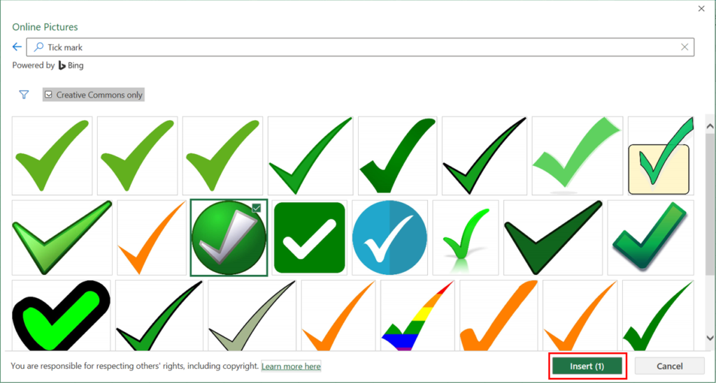
Let's not forget about the good old copy-paste functionality. If you’ve already got a tick mark somewhere in your workbook, or if you’ve found one online (just search for "tick symbol" and copy it!), you can simply click in the target cell, right-click, and select "Paste." Sometimes, the simplest solutions are the most effective. It’s like finding a perfectly ripe avocado – pure joy.

However, a word of caution: when you copy and paste a tick mark from external sources, Excel might treat it as a special character. This means that if you try to apply standard fonts to it, it might disappear or turn into something else entirely. So, if you’re pasting, make sure it behaves nicely. If not, resort to the Character Map or the Wingdings trick, which are more reliable within the Excel ecosystem.

Also, remember that the appearance of the tick can depend on the font installed on your computer and the version of Excel you're using. While Wingdings is pretty standard, sometimes you might encounter slight variations. It's like different accents for the same language – still understandable, but with a unique flair.

So, to recap our tick-tastic journey: you’ve got the manual route with Character Map, the font magic of Wingdings, the automation power of IF functions, and the visual flair of Conditional Formatting. Whichever method you choose, you're now equipped to conquer those pesky blank cells and bring a little order and visual delight to your spreadsheets. It’s not just about data anymore; it’s about data with a smile.

Think about all the possibilities! Project management sheets where you can visually track progress. Survey results where you can quickly tally choices. Inventory lists where you can mark items as received. The humble tick mark is a powerful little symbol, and now you know how to wield it. It's like you've unlocked a secret level in the game of Excel. Go forth and tick away, my friends! Your spreadsheets will thank you. And who knows, you might even start seeing ticks everywhere. Happy spreadsheeting!