How To Label An Axis In Excel

Alright, my fabulous friends! Let's talk about something that might sound as exciting as watching paint dry, but trust me, it's actually a secret weapon in your data-wrangling arsenal. We're diving headfirst into the thrilling world of… labeling axes in Excel!

Now, I know what you're thinking. "Axes? Labels? Is this going to require a PhD in advanced mathematics?" Absolutely not! Think of it more like… adding the perfect caption to your Instagram photo. You wouldn't just post a pic of your amazing brunch without telling everyone what you're munching on, right? Same goes for your charts!

Imagine you've painstakingly created this gorgeous, vibrant chart in Excel. You've got your data looking like a million bucks. But then, you glance at it, and it's just… there. A bunch of squiggly lines and numbers without context. It's like showing up to a party in a fabulous outfit but forgetting your name. People are confused! They're wondering, "What am I even looking at?"

This, my friends, is where the magic of axis labels swoops in to save the day! They're the friendly guides, the helpful signposts, the little voice that whispers, "Psst! This is the amount of pizza consumed per capita in the last fiscal quarter!" See? Suddenly, it's not just data; it's a story. And who doesn't love a good story?

So, How Do We Sprinkle This Data-Dressing?

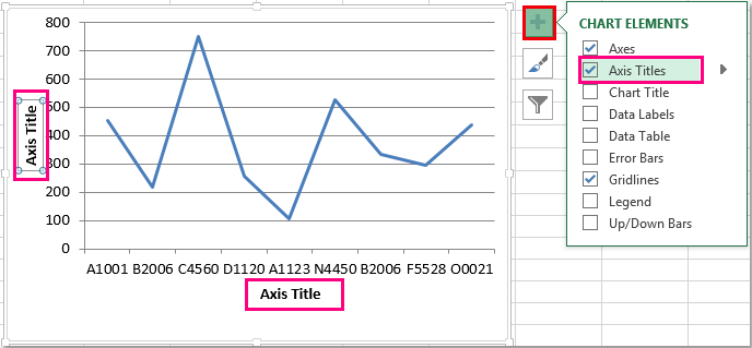
Let's get practical. You've got your chart selected, right? If not, gasp, click on it now! It's usually a simple click. Once it's highlighted, you'll see a few new tabs pop up at the top of your Excel window. We're looking for the ones that scream "Chart Tools" or something similar. Don't be shy, poke around!

Now, here's where the adventure really begins. Most of the time, you'll find a button or a menu option that says something like "Add Chart Element," "Chart Design," or "Layout." It's like a treasure chest of chart customization! Click on that, and then look for "Axis Titles." Ta-da! You've just unearthed a key component of data clarity.

Once you've clicked on "Axis Titles," you'll usually get a few options: "Primary Horizontal," "Primary Vertical," and maybe even "Secondary Horizontal" and "Secondary Vertical" if you're feeling fancy with multiple data sets. For starters, let's focus on the main two: the ones at the bottom (horizontal) and the ones on the side (vertical).

The Humble Horizontal Hero

Let's tackle the horizontal axis first. This is typically the one that tells you what you're measuring. Think of it as the "stuff" axis. Are we talking about months? Years? Names of your incredibly talented team members? Click on "Primary Horizontal" and then "Title Below Chart."

A little text box will appear, probably with some placeholder text like "Axis Title." Now, this is your moment to shine! Click on that text box, delete the boring placeholder, and type in something meaningful.

Let's say your chart shows sales figures over time. Instead of just a bunch of dates, you'd type in "Month of Sales" or "Fiscal Year." If it's about your company's amazing product launches, maybe "Product Name" or "Launch Date." See how much clearer that is? It’s like giving your chart glasses so it can see its own data properly!

The Vertical Voyager

Next up is the vertical axis. This is usually where you specify the quantity or value you're measuring. Think of it as the "how much" axis. Is it dollars? Units sold? Percentage of happiness achieved by your customers?

Click on "Axis Titles" again, but this time choose "Primary Vertical." You'll likely have an option for "Title Above Chart" or "Rotated Title." For a vertical axis, "Rotated Title" often looks the cleanest and most professional, but "Title Above Chart" can work too.

Again, click on the placeholder text and let your creativity flow. If your chart shows revenue, you'd type in "Revenue ($)" or "Sales Amount (USD)." If it's about customer satisfaction scores, maybe "Customer Satisfaction Score (out of 10)" or "Percentage of Positive Feedback."

And here's a little pro tip: don't forget your units! Including them in the axis title saves your audience from having to guess. It's the difference between saying "50" and saying "50 million dollars." Big difference, right?

Making It Pop (Optional, But Highly Recommended!)

Once you've got your basic labels in place, you can get a little more adventurous. Excel offers some fun formatting options. Want to make your axis titles a different color? Make them bold? Change the font? You can do all of that!

Just right-click on the axis title you've created, and look for "Format Axis Title." A panel will likely pop up on the side of your screen with tons of options. You can play with text fill, outline, text effects, and even text direction.

Think of it as accessorizing your chart! A pop of color here, a slightly larger font there. It’s all about making your data not just understandable, but also visually appealing. A good-looking chart is a chart that people want to look at.

Why is this so inspiring, you ask? Because you're taking raw, potentially overwhelming numbers and transforming them into a clear, digestible, and even beautiful representation of information. You're becoming a data storyteller, a visual communicator, and honestly, that’s a superpower!

Every time you label an axis, you're empowering yourself and your audience to understand the world a little better, one chart at a time. You're making data less intimidating and more accessible. You're making your reports more impactful and your presentations more engaging.

So, the next time you're faced with a chart that's mumbling its data secrets, remember the power of the axis label. Go forth, label with confidence, and watch your charts transform from mere collections of data points into compelling narratives that truly resonate. You've got this, and the world of data thanks you for making it clearer!