How Do You Type A Tick In Excel

So, the other day, I was knee-deep in a spreadsheet. You know, one of those ones that looks like a digital quilt, all cells and numbers and the looming dread of a misplaced decimal point. I was trying to create a little checklist, a “things to do” list, a “tasks completed” tracker. Standard stuff, right? And I thought, “Aha! The perfect visual indicator would be a little tick mark!” You know, that satisfying little checkmark that screams, “DONE!”

But then, the panic set in. How on earth do you type a tick in Excel? My fingers hovered over the keyboard, ready to unleash their typographic magic, but… nothing. Just the usual letters, numbers, and those pesky symbols that look vaguely like foreign currency. I’d seen them in other documents, those neat little ticks. Was it a special key combination? A secret handshake with my keyboard? My internal monologue went something like: “Is it Ctrl+Shift+T? Alt+Tick? Maybe I need to sacrifice a rubber chicken to the spreadsheet gods?” It sounds silly now, but in that moment, it felt like a genuine technological Everest.

This, my friends, is how the quest for the elusive Excel tick begins. It’s a journey many of us have embarked on, armed with nothing but a mild inconvenience and a desperate need for visual clarity. You see, Excel isn't just about crunching numbers; it's about presenting information in a way that doesn't make your eyes bleed. And sometimes, that means adding a little flair, a little visual cue. And what’s a better cue than a satisfying tick?

The Great Tick Hunt: Where Does It Hide?

After a few minutes of fruitless keyboard mashing (and maybe a frustrated sigh or two), I realized brute force wasn’t the answer. There had to be a more elegant solution. This is where the real detective work began. My brain, bless its heart, started to whir. Is it a character? A symbol? Does Excel have a hidden emoji keyboard I’m not privy to?

It turns out, the answer is a delightful mix of both, and understanding it is surprisingly simple. The most common and easiest way to get that glorious tick mark is through Excel’s extensive symbol library. Think of it as a secret treasure chest of characters that aren't readily available on your standard keyboard layout. You just need to know how to unlock it!

Option 1: The Symbol Explorer – Your Friendly Neighborhood Menu

This is probably the most straightforward method for beginners, and honestly, it’s the one I gravitate towards when I’m feeling a bit lazy or just want to be absolutely sure. Here’s the magic sequence:

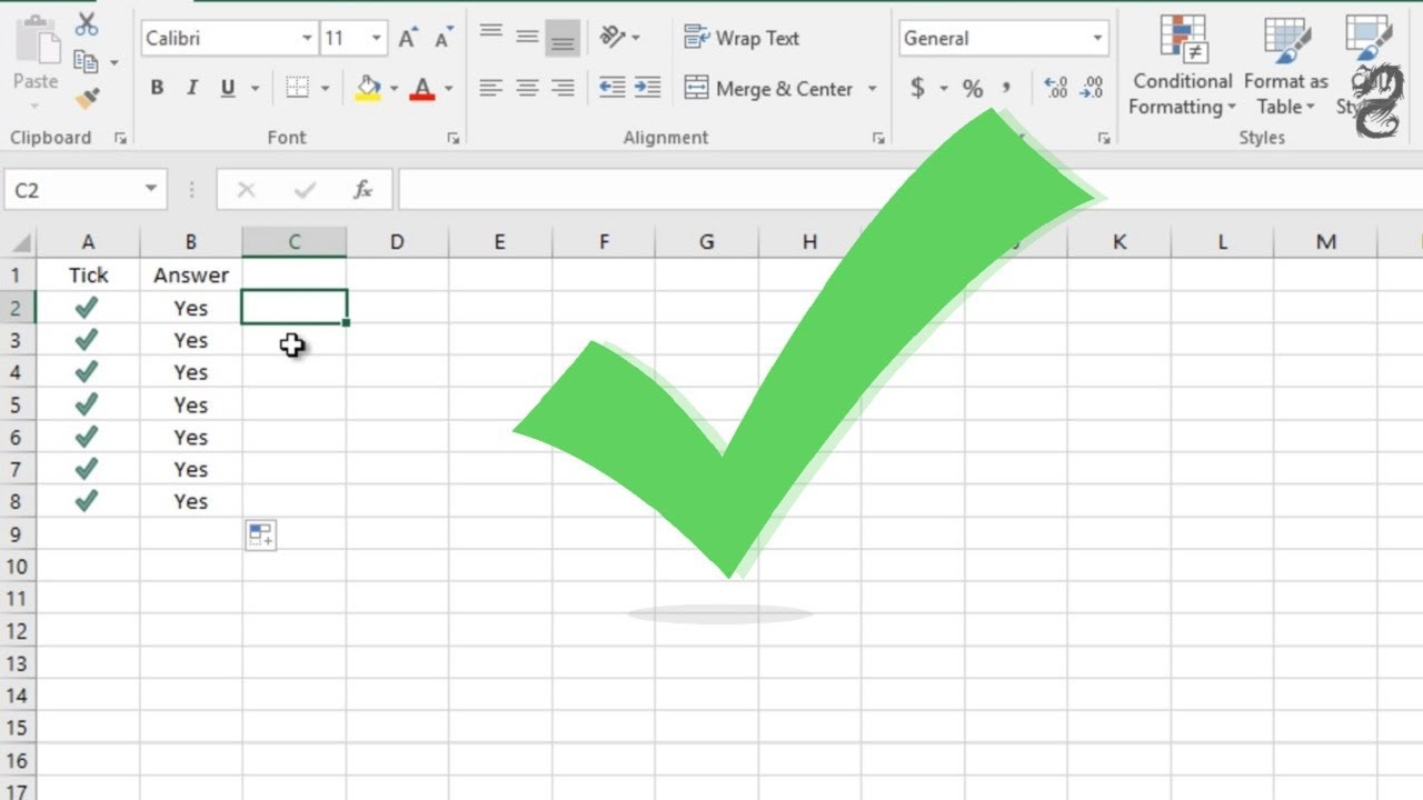
1. Click on the cell where you want your tick to appear. Obvious, I know, but hey, we’re being thorough!
2. Navigate to the Insert tab in Excel's ribbon. You know, the one with all the bells and whistles.
3. Look for the Symbols group. It’s usually lurking on the far right, like the shy kid at a party.
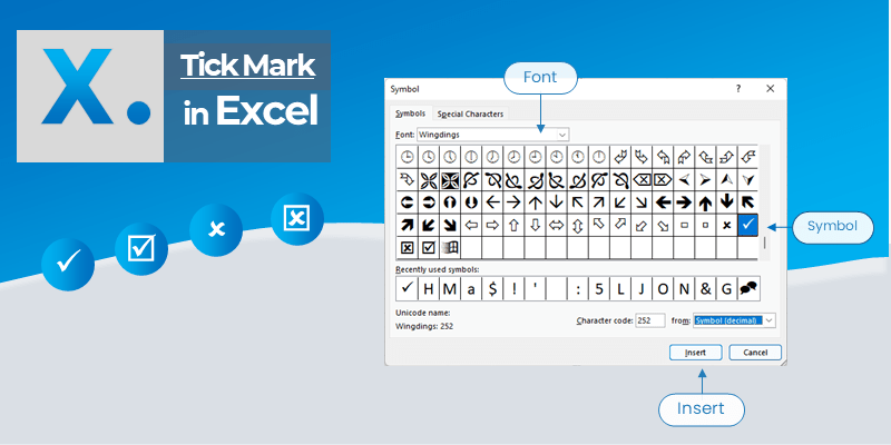
4. Click on Symbol. And BAM! You’re presented with the Symbol dialog box.

Now, this dialog box can look a little intimidating at first. It’s crammed with all sorts of characters. But don’t panic! Your tick is in there, I promise. You just need to know where to look. The key is to change the Font to something like Wingdings or Webdings. These fonts are specifically designed to contain a wealth of symbols and icons, rather than traditional letters.

Under the Wingdings font (try this one first, it’s usually the most populated with what you’re looking for), scroll through the characters. You’ll see all sorts of things – little airplanes, hands, silly faces. Keep scrolling. You’re looking for a character that resembles a tick or a checkmark. It’s usually pretty prominent. Once you find it, double-click on it, or select it and click Insert. And there you have it! Your tick, gracing your spreadsheet with its presence.

You can also do the same for the Webdings font, which has a slightly different, but equally useful, set of symbols. Sometimes one font has the exact tick you’re after, and sometimes the other does. It’s a bit of a lucky dip, but a very productive one!

Pro-tip: Once you’ve inserted a symbol, Excel often remembers which font you were using last. So, if you need more ticks, you won’t have to go through the font selection process again. Handy, right?

Option 2: The Keyboard Shortcut (For the Braver Souls)

Now, if you’re like me and sometimes enjoy a good keyboard shortcut, or if you’re using ticks so frequently that the Insert menu feels like a marathon, there’s an even faster way. This involves using the Alt code. Don’t worry, it’s not as technical as it sounds. It’s like a secret language for your computer!

Here’s the trick: you need to use your numeric keypad (the little block of numbers on the right side of most keyboards). If you’re on a laptop and don’t have a dedicated numeric keypad, you might need to enable the Num Lock and use the secondary number keys, which can be a little fiddly. But for those with a full keyboard, it’s a breeze.

Hold down the Alt key on the left side of your keyboard. While holding it down, type the specific number code on your numeric keypad. Then, release the Alt key. And voila!

For a tick mark, the most common and reliable Alt code is:

• Alt + 251 (This often gives you a checkmark symbol)

Important note: Make sure you are using the numeric keypad and not the number keys above your letter keys. This is where most people get tripped up. Seriously, I’ve seen it a hundred times. Your brain just goes to the top row numbers because they’re more visible. Nope! Gotta be the side ones!

Another variation you might encounter, depending on your system and the font you’re using, is:

• Alt + 0251 (Again, for a checkmark. The leading zero can sometimes make a difference.)

You might need to experiment a little to see which one works best for you and your specific version of Excel. It’s like a little treasure hunt for the perfect tick!

Personal anecdote time: The first time I successfully used an Alt code for a symbol, I felt like I’d unlocked a cheat code for life. I spent the next hour finding random symbols to type just for the sheer joy of it. My colleagues probably thought I’d lost it. "What are you doing?" they'd ask. "Just… exploring the untapped potential of my keyboard," I’d reply with a smug grin. Good times.

Option 3: The Character Map (For the Ultimate Control Freaks)

For those who truly want to understand the inner workings of their character sets, or if the previous methods are being stubborn, there's the Character Map tool. This is a built-in Windows utility that shows you every single character available in any given font.

To access it:

1. Press the Windows key + R to open the Run dialog box.
2. Type charmap and press Enter.

The Character Map will open. Here, you can select your font (again, try Wingdings or Webdings), and it will display all the available characters. Find your tick, select it, click Copy, and then paste it into your Excel cell. It’s a bit more manual than the other methods, but it gives you absolute precision and a fantastic overview of your font’s capabilities.

But Wait, There's More! (The "Smart" Tick)

Okay, so you’ve got your tick. But what if you want it to be a bit more… dynamic? What if you want it to appear automatically when you type something like "DONE" or when another cell is marked "Complete"? This is where things get a little more advanced, and we venture into the realm of Conditional Formatting or even a bit of simple VBA (Visual Basic for Applications) if you’re feeling brave.

Conditional Formatting: The "If This, Then That" of Ticks

This is a fantastic way to automate your ticks. Let’s say you have a column for "Status" and in another column (say, column B), you want a tick to appear if the status in column A is "Done". Here’s how you might do it:

1. Select the cells in column B where you want your ticks to appear.
2. Go to the Home tab.
3. Click on Conditional Formatting.
4. Choose New Rule.
5. Select "Use a formula to determine which cells to format".
6. In the formula box, you'll enter something like: =$A1="Done" (assuming your status is in cell A1 and you've selected from B1 downwards. Excel will automatically adjust the row number as you apply it to other cells).
7. Click the Format... button.
8. Go to the Font tab.
9. Change the Font to Wingdings.
10. In the Character preview, find and select your tick symbol.
11. Click OK on the Format Cells dialog box, and then OK again on the New Formatting Rule dialog box.

Now, whenever you type “Done” in column A, a tick will magically appear in column B! Isn’t that neat? It’s like having a tiny, invisible assistant who handles the tedious bits for you.

You can also use this for other scenarios. Maybe you want a red 'X' for "Not Done" and a green tick for "Complete". The possibilities are quite extensive!

The Irony of the Tick

It’s funny, isn’t it? We’re using these incredibly powerful tools, capable of complex calculations and data analysis, and yet, we spend time figuring out how to insert a simple little checkmark. It’s a testament to how important visual cues are, how much we crave that sense of completion, that little digital nod of approval.

The tick mark isn't just a symbol; it’s a tiny victory. It’s the culmination of effort, the marker of progress, the silent cheer of a job well done. And to be able to summon it with a few keystrokes or a quick menu click? That’s a small, but significant, win in the often-monotonous world of spreadsheets. So, the next time you’re in Excel, don’t be afraid to hunt for that tick. It’s more than just a character; it’s a little piece of typographic satisfaction.

Now go forth and tick all the things! Your spreadsheets will thank you for it. And your sanity, too. Believe me.